Alloy Manager

Calculation of the activity of individual components in alloys.

The development of this activity model was performed at the Oak Ridge National Laboratory.

The overall aim of the ORNL research task was to develop software modules to calculate activity of individual alloying elements as a function of concentration and temperature for a phase that is of interest. These calculated activity values are used in the OLI corrosion model for stability diagram calculations. The alloy systems that are of interest to current research project were copper alloys (Cu-Ni system), low-alloy steel (Fe-C-Mn), stainless steels (Fe-Cr-Ni-Mo-C), nickel alloys (Ni-Cr-Fe-Mo-C) and duplex stainless steels (Fe-Cr-Ni-Mo-C-N). The structure of the ORNL alloy module is depicted in Figure 1.

Methodology:

• The activity (a_i) of alloying element is related to its chemical potential (µ_i) as given by equation (1) [Lupis, 1983], (1).

	      (1)					

• The chemical potential in-turn is related to the molar free energy (G_m) and molar concentration (x_j) through the following relation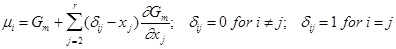,(2).

	      (2)

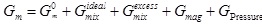
• The molar free energy of the alloys as a function of alloying element concentration were described using sub lattice model [Sundman et al, 1985 and Saunders & Miodownik, 1998] and is given by the following formulation,(3).

             (3)

In the above equation, is the contribution due to pure components [Dinsdale, 1991], is the ideal mixing contribution, is the contribution due to non-ideal mixing, is the contribution to magnetic Gibbs energy, and is the contribution due to pressure term [Saunders and Miodownik, 1998].

Results: Published thermodynamic data for constituent binary systems (e.g Fe-C, Gustafson, 1985), ternary systems (e.g. Fe-Cr-C by Andersson, 1988) and quaternary systems (e.g. Cr-Fr-N-Ni by Frisk, 1991) were used to develop the software module for stainless steels, nickel alloys and duplex steels. The software modules were designed to calculate the activity of constituent alloying elements in both austenite (face-centered cubic crystal structure) and ferrite (body-centered cubic crystal structure) as a function of concentration and temperature. The software modules were evaluated with ThermoCalc® calculations for accuracy [Sundman et al, 1985]. The calculations shown in Fig. 2 show good agreement with ThermoCalc® predictions. In addition, the plots show the activity of Mo in BCC phase will be many orders of magnitude higher than that in FCC phase. The above results are significant since the corrosion stability diagrams can be evaluated for different phases with the same compositions.

Incorporation of the Alloy Model into Stability Diagram Software

The alloy thermodynamic modules have been integrated with the software for generating stability diagrams. For this purpose, the stability diagram code has been revised to incorporate a Gibbs energy model not only for the aqueous phase, but also for the solid (alloy) phase. In this section, we describe the algorithm for generating stability diagrams for alloys.

A stability diagram for a given physical system can be viewed as a superposition of elementary diagrams for the redox subsystems that make up the system of interest. For example, a system composed of a Fe-Ni alloy in an H₂S solution can be treated as a superposition of five redox subsystems defined as:

• (1) All species containing Fe in any possible oxidation state (0, +2, +3 and +6)
• (2) All species with Ni in the 0, +2, +3 and +4 oxidation states;
• (3) All species with S in any possible oxidation state ranging from -2 to +8;
• (4) All species with H in the 0 and +1 oxidation state and

    All species with O in the -2, 0 and, possibly, -1 oxidation states.

Thus, each redox subsystem is associated with an element that can exist in two or more oxidation states. Each of the elementary redox subsystems is characterized by a set of equations that may occur between the species that belong to the subsystem. The subsystems are interdependent because the reactions in each subsystem involve species that belong to more than one subsystem. However, the relationships between the potential and activities or concentrations of species can be separately plotted for each subsystem. For example, the classical Pourbaix diagrams (1966) are shown as superposition of three elementary diagrams, i.e., one for a redox subsystem containing a selected metal, one for the oxygen subsystem and one for the hydrogen subsystem. The latter two subsystems are usually represented by single lines that correspond to the H⁺/H₂ and O₂/H₂O equilibria. 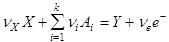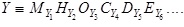To compute a stability diagram for each redox subsystem, it is necessary to enumerate all distinct chemical species that belong to this subsystem. Each of these species contains the particular element that is associated with the subsystem. Then, equilibrium equations are written between all species in the subsystem. If the number of species is n, then n(n-1)/2 reactions are defined. A reaction between the species X and Y is written as

         (4)                                              			

where A_i (i = 1,...,k) are the basis species that are necessary to define equilibrium equations between all species in the redox subsystem and V_i are the stoichiometric coefficients. For convenience, each reaction is normalized so that the stoichiometric coefficient for the right-hand side species (Y) is equal to 1.

To establish a general algorithm for defining the basis species A_i we note that the species X and Y from equation (4) can be represented as

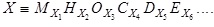         (5)

         (6)

where M is the element that is associated with the redox subsystem, H and O are the usual symbols for hydrogen and oxygen, respectively, and C, D, E,... are the additional elements that exist in the species X and Y. For the purpose of defining the basis species, we separately treat elements in different oxidation states. For example, C and D can represent the same element in two different oxidation states. The basis species are then defined as the species that contain H, O, C, D, E, etc., but do not contain M. Although this definition allows considerable flexibility in choosing the basis species A_i, additional rules are introduced to simplify the algorithm:

(a) H+ is always the basis species that contains H; (b) H2O is always the basis species that contains O; (c) The basis species containing C, D, E, etc. are selected so that they contain the minimum possible number of hydrogen and oxygen atoms in addition to C, D, E,... .

To illustrate the selection of basis species, let us consider two examples. In a system composed of Cu, H₂O and NH₃, the species in the copper-containing redox subsystem are copper hydroxides, oxides and complexes formed by Cu with the OH^- and NH₃ groups. Therefore, the general formula for the species is where N^-3 denotes N in the -3 oxidation state. Thus, the basis species for constructing reactions (5) are H⁺, H₂O and NH_3(aq). In a system composed of iron, water and sulfur-bearing compounds, the species in the iron subsystem are iron hydroxides, oxides, hydroxycomplexes, sulfides, polysulfides and sulfates. The general formula for the species is then and the basis species are H⁺, H₂O, S^2-, S⁰_(s) and SO₄^2-. After selecting the basis species, the stoichiometric coefficients in equation (5) are determined by balancing the elements M, H, O, C, D, E, etc. Finally, the number of electrons (V_e) is found by balancing the charges on the right- and left-hand sides of equation (5).

The selection of basis species is slightly more complicated in cases when not only the element M (cf. eqs. 5 and 6) is subject to redox equilibria, but also some of the elements C, D, E, etc. can enter into their own redox equilibria. A typical example is the iron-water-sulfur system, in which both iron and sulfur can exist in several oxidation states. In the iron-containing subsystem, the transformations between the various species can involve the oxidation and reduction of either iron or sulfur or both. In such cases, the basis species are modified in a two-step procedure:

First, it is determined which basis species are stable in which area of the stability diagram and only the stable species are retained in the basis and the remaining ones are deleted. The deleted species are not taken into account for constructing the equilibrium equations (4) but, otherwise, they are kept in the system.

Since different basis species can be stable in various areas of a stability diagram, the steps (1) and (2) are usually repeated in as many areas of the diagram as necessary. This procedure ensures that only the stable basis species are included in the reactions. For example, elemental sulfur (S⁰) is stable only in a certain fraction of the E-pH plane. Therefore, S⁰ is used as a basis species to construct the reactions for the iron subsystem only when S⁰ stable, i.e., when solid sulfur can exist in a finite amount.

The proposed procedure for constructing equilibrium equations is considerably more complicated than the techniques proposed in the literature in conjunction with the classical Pourbaix diagrams (1966). However, it makes it possible to include chemical transformations of any complexity and is not limited to those involving H⁺ and H₂O.

Equilibrium lines. In the classical Pourbaix diagrams, each line represents the equilibrium between two chemical species for a given activity. Since the activity of dissolved species is assumed a priori, it is possible to derive analytical expressions for the equilibrium lines. Such expressions give pH values for the equilibrium between two species that do not undergo a redox reaction and express the potential as a linear function of pH for redox transformations. In the real-solution stability diagrams, the activities of all species vary because of the changing amounts of input species (such as an acid or a base used to adjust pH). Activity coefficients are nonlinear functions of composition and may cause nonlinearities in the equilibrium lines. Therefore, it is not possible to derive analytical expressions for the equilibrium lines. Instead, a certain number of points on the equilibrium lines has to be numerically computed. The points can be further interpolated to obtain an equilibrium line.

Stability diagrams are constructed by performing a simulated titration with reactants that are appropriate for varying the independent variable of interest. If pH is the independent variable, two reactants - an acid and a base - are selected for the simulated titration. First, decreasing amounts of an acid are added to cover the acidic pH range in regular increments. Then, increasing amounts of a base are added to cover the basic pH range. If the influence of a complexing or other reactive species is studied, the input amount of this species or its equilibrium concentration can be chosen as possible independent variables. Then, a compound containing this species is added in regular increments. For each amount of the added reactant, equilibrium compositions of various species in the aqueous phase are computed. At the same time, the activity coefficients are obtained. The concentrations and activity coefficients are further used to calculate the points on the equilibrium lines as explained below. In typical diagrams, it is sufficient to calculate between 20 and 30 points on the equilibrium lines provided that they are evenly spaced to cover a full range of the selected independent variable.

Chemical reactions. The chemical reactions are defined as the ones for which the number of electrons V_e (cf. eq. [4]) is zero. Since the chemical reactions are independent of the potential, they are represented on stability diagrams as vertical lines. In this case, an equation for the affinity A of reaction (4) is written as

    = (7)

where K is the equilibrium constant of reaction (5) and a_i denotes the activity of species i. The equilibrium constant is calculated from the standard-state Gibbs energies as

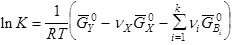           (8)                                    				

The activities of dissolved species are related to the molalities m_i and activity coefficients by

     	 (9)				                                              

At equilibrium, the affinity of the reaction is equal to zero. In the particular case when reaction (5) occurs between an aqueous and a solid species, the equilibrium corresponds to the precipitation of an infinitesimal amount of the solid phase. If reaction (5) is between two aqueous species, the point of zero affinity corresponds to equal activities of the species X and Y. If the affinity is positive, the species on the right-hand side of equation (5) predominates. Similarly, if the affinity is negative, the species on the left-hand side is predominant. The species that is not predominant may be either completely absent (which is usually the case for precipitation equilibria) or may be present in smaller quantities than the predominant species.

The values of the affinity of the chemical reaction (equation [7]) are calculated for each step of the simulated titration. This allows us to construct a discrete function, i.e.,

       (10)                                               			

where var_p is the independent variable (such as pH or concentration of a complexing agent) at the point p of the simulated titration, A_p is the corresponding value of the affinity of reaction (8) and N is the total number of steps in the simulated titration. The function (10) is then interpolated using cubic splines. The interpolating function is used to find the independent variable var₀ for which A=0., i.e.,

             (11)                         						

The independent variables found in this way are later used as the coordinates of the vertical lines on the stability diagram. After finding the root of equation (11), it is necessary to check which one of the two species is more stable at var>var₀ and at var<var₀. This is easily accomplished by checking the sign of the function f(var). For particular pairs of species, the root of equation (11) may not be found, which means that one of the species is more stable in the entire range of independent variables. The analysis of chemical equilibrium equations is repeated for each pair of species, for which the number of electrons V_e is zero. Thus, a collection of vertical boundaries in the stability diagram is established.

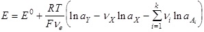
Electrochemical reactions. In the case of electrochemical reactions, the number of electrons V_e in equation (5) is not equal to zero. In this case, equilibrium potentials that correspond to reaction (5) are computed for each pair of species X and Y, i.e.,

             (12)  			

where R is the gas constant, F is the Faraday constant and E⁰ is related to the standard-state Gibbs energies by

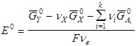             (13)                     				

In eq. (12), the activities a_i pertain to either solution or solid species. For solution species, they are calculated from the thermodynamic model of aqueous solutions (Rafal et al., 1995). For solid species that are components of alloys, the thermodynamic model of alloys (subtask 1.1) is used. For pure solid species, the activity is equal to one. The values of the potential are obtained from eqs. (12-13) for each step of the simulated titration and used to construct a discrete function of the independent variable, i.e.,

     (14)
                                                    				

where var_p is the independent variable at the point p of the simulated titration and E_p is the value of the potential calculated from equation (12). The function (14) is then interpolated using cubic splines.

Areas of predominance. After determining the equilibrium lines that correspond to chemical and electrochemical equilibria, areas of predominance are computed for each species in the redox subsystem of interest. For each species, four classes of boundaries are differentiated:

Upper boundaries, which correspond to equilibria with other species that are in higher oxidation states. If the number of electrons V_e in equation (4) is positive, the line determined by equation (12) will be an upper boundary for the species X. Conversely, if V_e<0, the line determined by equation (12) will be an upper boundary for the species Y. Lower boundaries, which correspond to equilibria with other species that are in lower oxidation states. The line determined by equation (12) will be a lower boundary for the species X if V_e<0 or a lower boundary for Y if V_e>0.

Right-hand side boundaries, which mean that the species under consideration is predominant for independent variables that are lower than the root var₀ of equation (10). Left-hand side boundaries, which mean that the species is predominant for independent variables that are greater than var₀. The sign of the affinity (equation [10]) is used to determine whether a vertical boundary is a right- or left-hand side boundary.

In general, there can be several boundaries of each kind. Therefore, an automatic procedure is set up to find intersection points between the boundaries and determine which ones are active (e.g., the lowest upper boundary and the highest lower boundary will be active for any given independent variable). In the case of systems in which the basis species are adjusted depending on the stability of the potential ligands, the stability areas of the ligands are determined prior to the calculation of the predominance areas for the redox subsystem of interest. Then, the predominance areas for the redox subsystem are separately determined within the stability area of each ligand. Despite the separate determination of the predominance areas in different parts of the diagram, there is always a smooth transition at the boundaries between the ligand stability areas because the reaction equilibria, concentrations and activity coefficients in each ligand stability area are interdependent and mutually consistent.

Thus, stability diagrams can be now generated for common engineering alloys in aqueous environments. Also, the data bank of thermodynamic properties has been extended to include mixed metal oxides, which are responsible for passivity in stainless steels and nickel-based alloys.

This was former Tip52